library(tidyverse)
ggplot(mpg) +
geom_jitter(aes(cty, hwy), size = 4, alpha = 0.5) 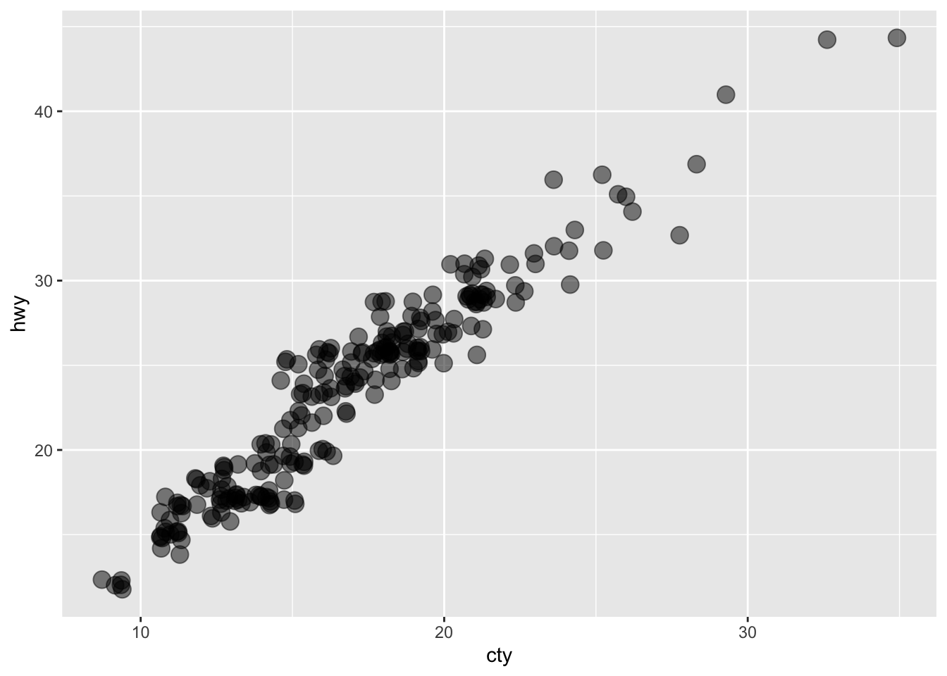
Lorem ipsum dolor sit amet, consectetur adipiscing elit. Nam suscipit est nec dui eleifend, at dictum elit ullamcorper. Aliquam feugiat dictum bibendum. Praesent fermentum laoreet quam, cursus volutpat odio dapibus in. Fusce luctus porttitor vehicula. Donec ac tortor nisi. Donec at lectus tortor. Morbi tempor, nibh non euismod viverra, metus arcu aliquet elit, sed fringilla urna leo vel purus.
Lorem ipsum dolor sit amet, consectetur adipiscing elit. Nam suscipit est nec dui eleifend, at dictum elit ullamcorper. Aliquam feugiat dictum bibendum. Praesent fermentum laoreet quam, cursus volutpat odio dapibus in. Fusce luctus porttitor vehicula. Donec ac tortor nisi. Donec at lectus tortor. Morbi tempor, nibh non euismod viverra, metus arcu aliquet elit, sed fringilla urna leo vel purus.
This is inline code plus a small code chunk.
library(tidyverse)
ggplot(mpg) +
geom_jitter(aes(cty, hwy), size = 4, alpha = 0.5)
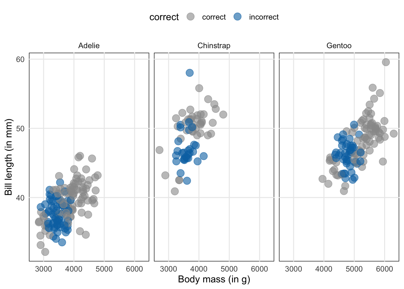
preds_lm %>%
  ggplot(aes(body_mass_g, bill_length_mm, col = correct)) +
  geom_jitter(size = 4, alpha = 0.6) +
  facet_wrap(vars(species)) +
  scale_color_manual(values = c('grey60', thematic::okabe_ito(3)[3])) +
  scale_x_continuous(breaks = seq(3000, 6000, 1000)) +
  theme_minimal(base_size = 12) +
  theme(
    legend.position = 'top',
    panel.background = element_rect(color = 'black'),
    panel.grid.minor = element_blank()
  ) +
  labs(
    x = 'Body mass (in g)',
    y = 'Bill length (in mm)'
  )
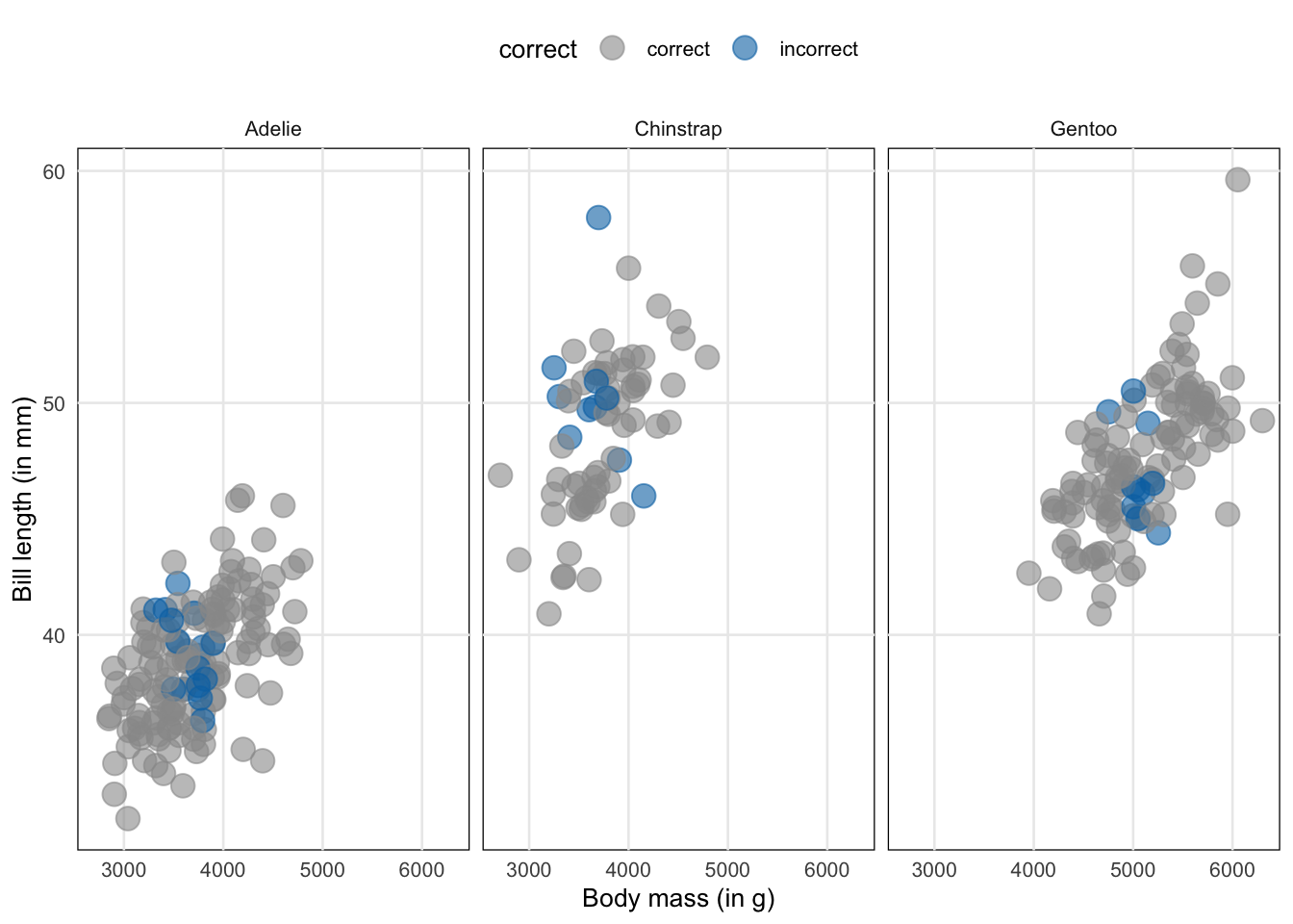
glm.mod <- glm(sex ~ body_mass_g + bill_length_mm + species, family = binomial, data = dat)
preds <- dat %>%
  mutate(
    prob.fit = glm.mod$fitted.values,
    prediction = if_else(prob.fit > 0.5, 'male', 'female'),
    correct = if_else(sex == prediction, 'correct', 'incorrect')
  )
preds %>%
  ggplot(aes(body_mass_g, bill_length_mm, col = correct)) +
  geom_jitter(size = 4, alpha = 0.6) +
  facet_wrap(vars(species)) +
  scale_x_continuous(breaks = seq(3000, 6000, 1000)) +
  scale_color_manual(values = c('grey60', thematic::okabe_ito(3)[3])) +
  theme_minimal(base_size = 10) +
  theme(
    legend.position = 'top',
    panel.background = element_rect(color = 'black'),
    panel.grid.minor = element_blank()
  ) +
  labs(
    x = 'Body mass (in g)',
    y = 'Bill length (in mm)'
  )
geom_density(
  mapping = NULL,
  data = NULL,
  stat = "density",
  position = "identity",
  ...,
  na.rm = FALSE,
  orientation = NA,
  show.legend = NA,
  inherit.aes = TRUE,
  outline.type = "upper"
)stat_density(
mapping = NULL,
data = NULL,
geom = "area",
position = "stack",
...,
bw = "nrd0",
adjust = 1,
kernel = "gaussian",
n = 512,
trim = FALSE,
na.rm = FALSE,
orientation = NA,
show.legend = NA,
inherit.aes = TRUE
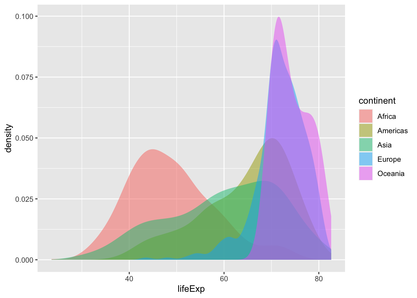
)ggplot(data = gapminder::gapminder, mapping = aes(x = lifeExp, fill = continent)) +
stat_density(position = "identity", alpha = 0.5)